
Creating a Decision tree
This section will teach you how to make a decision tree in kazAnova. Decision trees are algorithms that attempt to find the propensity of an event to occur by filtering and sub-filtering the data set many times. More specifically we pick a statistic that measures predictiveness such Gini or Chisquare or something else and we calculate it for all the variables one by one versus a Target variable. The one that has the highest statistic will sit on top of the tree and in our case it will be the DISEASE variable that had the highest predictability measures in all categories. Then for each one of the distinct values of this variable (e.g when DISEASE=CANCER) we filter our set (e.g. we pick only the cases that had CANCER) and we calculate again the statistics for all variables and we pick the one with the highest value that will now sit in the second layer. We do this for all the distinct values of DISEASE. With this method and by adding variables we start explaining information that we could not explain only with the first variable. The process can become quite complicated as we move to 3 or 4 layers down.
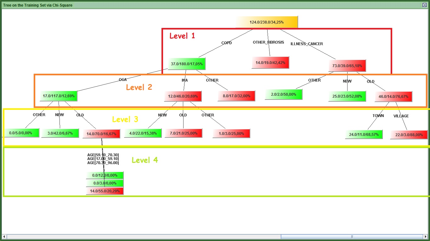
Image: Tree levels
One problem associated with trees is they can become too big to interpret. kazAnova can control how many levels (or layers) of variables you can add though. Another problem is that if the tree becomes too complicated and deep, it becomes too specific on the training set, it gets over fitted. Imagine over-fitting like instead of trying to find groups of characteristics that constitute a specific behavior, you say if a person has one blue and one green eye, 3 white hairs, a tattoo with kazAnova’s logo on his left knee, 3 pounds in the right pocket inside his Y-brand jacket that bought it from Z store at a Tuesday when it was raining and the temperature was -2 C, then this person is good. Such a combination might be found in the training set, but it is very unlikely to happen again. An over fitted model will build such criteria (as a general concept but not so dramatic!) to decide if a person is good or bad. Therefore you need to stop the tree’s expansion before it becomes too big and you need to remember that the tree is very greedy and loves gossip so that it will try to get to very bottom if you don’t put block.
In the scorecard section, we used categorical (and string) variables to build the model. The tree does not have a limitation, you could use categorical or no variables. Additionally, you do not need to do any binning as the algorithm will do that for you, but you need to specify the maximum number of bins you want to have. For example if you set maximum bins to 3, it will make certain that all variables , basically the ones with more distinct values such as DISEASE (that had 5) will have only 3 when running the algorithm by merging some values. This process also controls the expansion of the tree as you have less distinct values to worry about. There are a couple of more tools to control the expansion of the tree, but I will mention it along the tutorial.
You can now use the same file you have been using in the tutorial or re-open the first version that that was not manipulated. Up to you, it makes no difference which set you use, because we will use only the default variables.
We need to create a partition variable at this point, if you have one from before then you can skip this part or you can just do it again so as to make certain that you know how to do it:
- Go to the Pre-process tab in the menu bar and press “Sampling”
 .
. - In the new frame, change the name in the second text field from the top from “partition001” to partition_tree.
- Press “Compute”.
We are ready to begin the tree algorithm now, but remember that you will get slightly different results from me because you have different partition :
- Go to the Scorecard tab in the menu bar and press “Tree Model”
 .
. - In the new window that appears, select Target from the left or type Target in the first text field from the top.
- In the third (right) column select partition_tree or your partition variable if it is different. Alternatively you could type partition_tree in the third text field from the top.
- In the middle column, you could do a multiple selection. Left click on the variable TYPE, hold shift and press up to where you want your selection to be expanded. If the set is in the same order I gave it to you and you did not make any chemical experiments, then click on INSTITUTION(While holding Shift). Else type
TYPE,REGION,INSURANCE,QUANTITY,HOURS,SEASON,DISEASE,AGE,INSTITUTIONin the second field from the top to include all these variables. You could also select them all one by one, but it is much faster this way. You may refer to the figure under this section to see how I did it.
- Leave the fourth field to 4 as it is. This will allow the tree to expand up to the fourth level if no other constrain stops it. For example if you put 3, the tree will not expand beyond the third level.
- Change the fifth text field from 50 to 30. Essentially with this we tell kazA that we don’t want to split a group if there are less than 30 cases. Tweaking different values here can help you to prevent over fitting.
- Note the last menu that has chi Square. This will be the main statistic when trying to order the variables. Do not change it in order to get more similar results.
- Leave everything else as is and press “Confirm”.
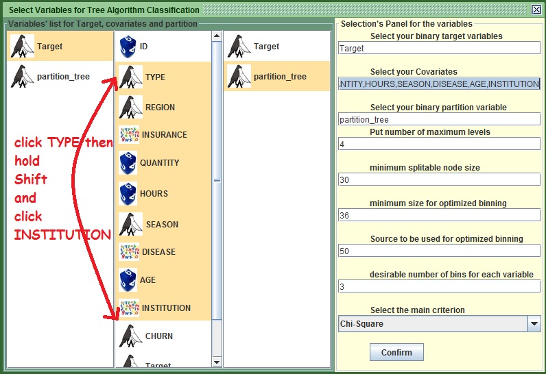
Image: Tree's preparation panel
Have a look at the highlevel sections of the tree’s outputs:
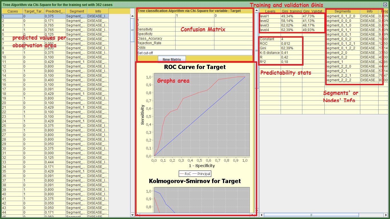
Image: Tree's Output
Starting from the right panel you can see the ginis of training and validation at each level. If you decide to stop your tree at x level, you will get the gini of training and validation in that level. In my case for example, If I want to stop my tree at level 2, the level 2 gini of the training set is 58.14% and the validation is 41.13%. This difference is huge and probably a product of over fitting. Generally a difference higher than 2 %or 3% at all levels between the 2 sets is a cause for concern, depending always on the data size. In level 4 my figures look better and the difference between training and validation is smaller. This suggests that I should use all the 4 levels of the tree for my prediction. However this modeling approach does not seem to be very successful.
You have heard a lot about the tree, but you haven’t seen one so far and I endanger myself of being called a liar. For this reason only:
- In the middle panel scroll down until you reach the end.
- Press the button “Visualize”.
- In the new frame that appears, double click on the header of the frame (the green part) in order to make the horizontal bar to appear.
- Once the bar appears, go right and left to have a good view of the tree.
- If you want to push everything into the same viewport, you have to do it manually. Press and hold left click and hold it to create a perimeter area that includes some nodes (squares) of the tree, like in the figure below, then release the button. You will notice that the nodes you included in the area appear differently because they are selected.
- Hold left click by selecting one of the nodes and move the area right or wherever you want. With this method you can compact the whole tree in a small area and shape it as you like.
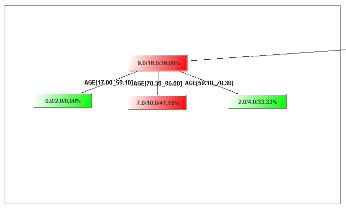
Image:Nodes' selection
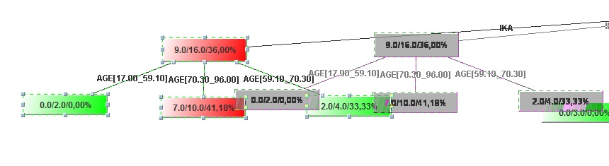
Image:Move selection
Below you can visualize the top level of my tree:
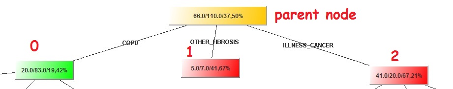
Image:Top tree level
The top node with the yellowish color as every other node has 3 figures in this format num/num/percent. What the “Father” of all nodes tell us based on my graph is that there are 176 (66 + 110) cases in our validation set. Of those 176, 66 or 37.50% churned. This Node has three children. One child is green and the other two are red (I am wondering what is the color of the mother so as to produce children with such color diversity!). The Green color implies that the percentage of churners (that have a value of 1) is less than the father (19.42% < 37.50%). Similarly the red color implies the child has surpassed the father in propensity to churn, but generally it follows his foodsteps.
One last thing, I have put some numbers on the top of the children nodes. Always the left most is labeled as “0” and all the other will have incrementally more (e.g. the second will be “1” and if there is a third that will be “2” and so on). Some of these 3 children (the “0” and the “2” in my case) made their own families and have children of their own. Let’s take for example those that the DISEASE is COPD (left). If I want to refer to the left most child that it has, I will refer to it as 0_0. If I want to refer to its third one then it would be 0_2 and so on. Although you can see the value of the variables, (e.g. COPD) you cannot see the variable names (e.g. DISEASE), but you can see that elsewhere.
Now we learnt how to interpret the nodes, but it takes time to feel comfortable with the output therefore do not feel disappointed if you find it a bit difficult. Back to the right panel, you can see the predictability statistics. What you need to be aware of is that the graphs and all the charts as well as all the predictability statistics refer to the last level of the validation set. The only exception is the area under ROC statistic (labeled as ROC) and the Gini that is displayed in the predictability stats. These two refer to the fourth level of the training set. I left it as such, because you can see the Gini from the above section that shows the comparison between training and validation.
By focusing on the segments’ node info section, you can see the details for each one of the segments (nodes) of the tree based on the training set. See my table:
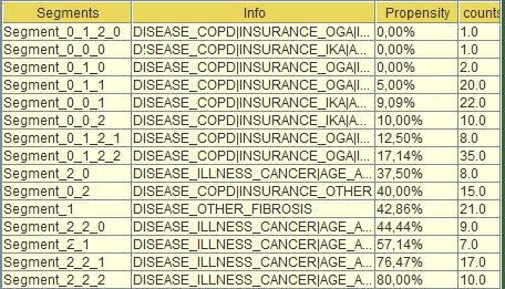
Image:Segments' section
Segment_0_0_0 (second from the top in the table) refers to the left most child of the tree that sits in the third level. You can see if you look at the info tab (next column) what each one of these “0” are . E.G. at top level if DISEASE = COPD “|”(this means “and”) INSURANCE=IKA and AGE is between [17-59] (see below) this is segment_0_0_0.
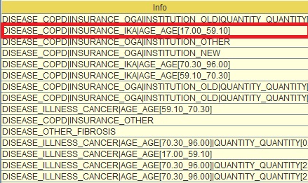
Image:Segments' Info section
This segment had propensity to churn 0% (third column) but there was only 1 person with this combination (fourth column) which implies that the tree became too specific in that case. You can then go back to the tree (by pressing "Visualize" again) and see if this 0% propensity is verified or is close enough for the validation set and whether you had significantly more people sitting in that segment. The propensity to pay is also the score in the tree process.
The Left panel, similarly with the Scorecard, shows in which segment each one of the observations (data rows) sits, displays their info and their propensity to pay (Predicted_Value) as the latter appears in the right panel for each segment.
The middle panel is exactly the same as in the scorecard output; the only difference here is that instead of scores you have the propensity to pay. You may export the results with the button “Export” that is located and the end of the middle panel. Then you can attach it to your main set via preprocess and Manipulation![]() .
.
Generally, in terms of modeling, my tree was not a very good one as the differences between training and validation set were very substantial. This happened because the set is rather small. Some actions to consider is to increase the minimum split able node size (where we changed the value to 30), decrease the number of bins (e.g from 3 to 2), decrease the number of levels and if the situation has not changed then re-sample (e.g. create new partition variable).
That is the end of tutorial 5. Tutorial 6 will show you how to use cross tabulation and how to create new variables with the M language. This tutorial can be considered as an extra and it is only if you want to dive deeper into kazAnova world, otherwise you have everything you need and feel confident to create your own models and save your business from the economic recession or just have some fun.