Preparing the Variables
In previous section we came to know our variables better, however if we are to create a scorecard, we will need our variables to be categorical. We need to create Groups in the variables AGE, HOURS and QUANTITY. Also because our set is small, it would be a good idea to merge some of the values of our String Variables (like DISEASE) so as to increase their impact.
Same as before:
- Go to the Graphs tab in the menu bar and press Histogram
 .
. - On the left of the two columns, select AGE or Type AGE in the first text field from the top and on the right column select Target or type Target in the second text from the top.
- Leave the number of bins to 10 and Press confirm.
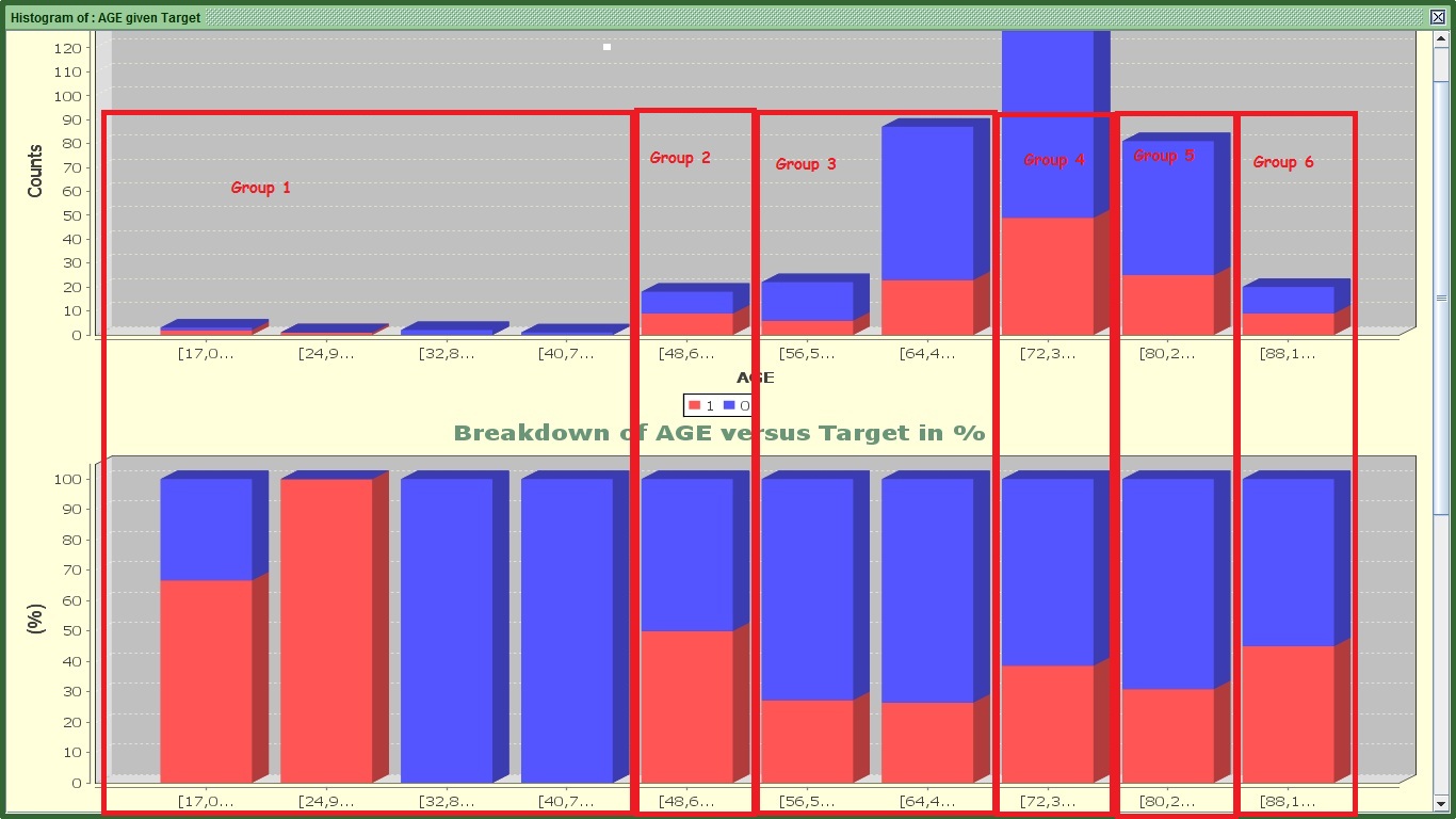
Image:Histogram of AGE versus Target with made-up segments
Something you need to know is that regression analysis (commonly used to create scorecards) attempts to find linear relationships. This means it will always try to find something like “the higher the age…the higher the propensity to churn” or “the fewer the HOURS … the lower the propensity to pay”. You can clearly see from the graph above that it does not work like that as very young people have high propensity to churn, the slightly older groups do not have high propensity , but middle aged groups have higher propensity again, that lessens again once we move to AGE 56 to 70 and then increases and again drops! If we don’t help the algorithm (in that case regression) to pick up those groups we will lose great information in explaining the target by saying “the older…the higher propensity”. Leave this chart open as we will revisit it very soon.
To visualize this problem in terms of predictiveness:
- Go to the Pre-process tab in the menu bar and press Gini
 .
. - On the left of the two columns, select AGE or type AGE in the first text field from the top and on the right column select Target or type Target in the second text from the top.
- Press "Generate".
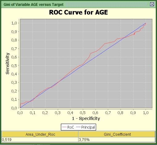
Image:Gini of AGE versus Targetun segmented
Because we have not set up groups in AGE, by attempting to find a relationship such as “the older…the higher” gives a very poor Gini and results in loss of information regarding how the target takes the values of 1 or 0. The fact that you see the curve going down the blue line means that for some age groups the relationship is negative (e.g. as “the older…the lesser”).
Going back to the first graph that I told you not to close it , you can see that I have created some segments or groups of similar propensity levels, focusing always on the second from the 3 graphs. I know that the first segment has completely extreme propensity levels, but the population is very small to be able to justify this propensity. Additionally, the company does not seem to have many subscribers in that category so it is OK to leave it as such.
Let’s create the same bins manually:
- Go to the Pre-process tab in the menu bar and press bin
 .
. - In the only available column, select AGE or Type AGE in the second text field from the top.
- Change the name of the potential new variable in the first text field from the top to AGE_USER from AGE_derived.
- Press the third button from the top “User_Defined”.
- On the only available column, select Target or Type Target in the first text field from the top.
- Under the Historgram of AGE and under the tab “split point”, double click inside the white cell and put our first threshold 48.5 (so as to make certain that AGE 48 is within this group).
- Click somewhere else to deselect that cell and press the “ADD” button.
- See that the graph has changed and you can also visualize the information value that this variable would have if it was created now- in its current state. You can also see how many churners and non-churners appear in each group.
- Double click inside the new cell that appeared under “split point” that has the maximum value of AGE (in this case 96).
- Replace it with the next threshold that is 56.4 (so that AGE 56 is definitely in that group), Click somewhere else to deselect that cell and press “ADD”.
- Do the same thing for the following thresholds, 72.2, 80.1, 88.05, always adding the value in the last cell under “split point”.
- The figure should now look like that, having a more decent Information value.
- Press the last button “Apply” to create your variable and close the pre-process tab.
- To illustrate what you have done in terms of capturing this underlying information for the target, Go to the Preprocess tab in the menu bar and press Gini .
- On the left of the two columns, select AGE_USER (the new variable) or type USER in the first text field from the top and on the right column select Target or type Target in the second text from the top.
- Press Generate.
- Save.
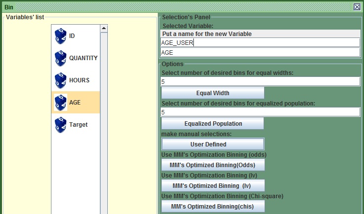
Image:Process of binning AGE manually
In the new window that appears:
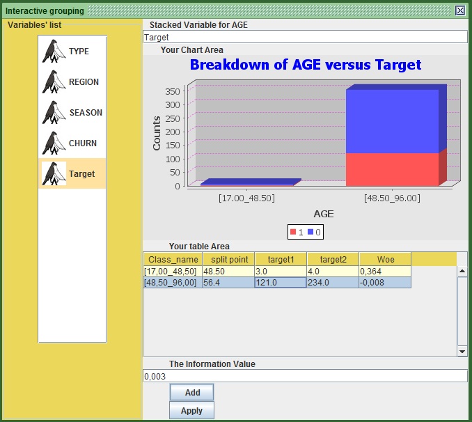
Image:Interactive Grouping of AGE
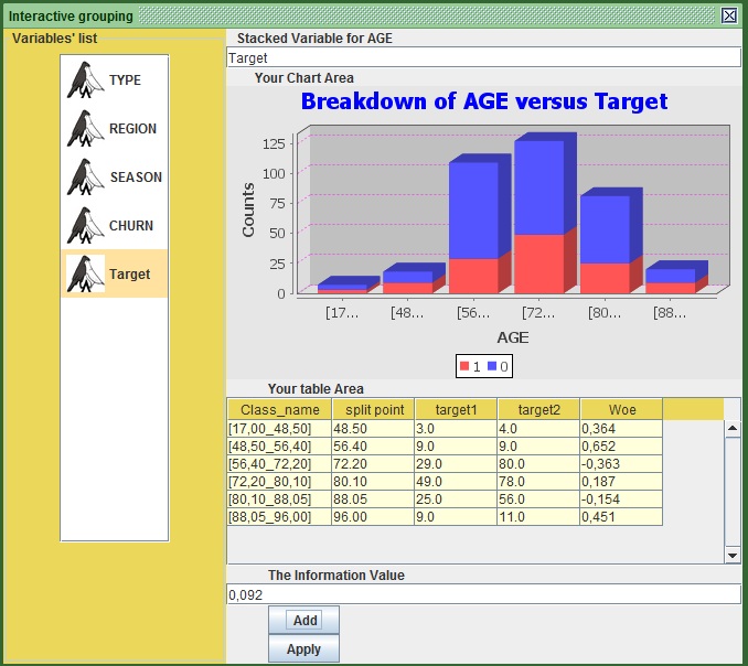
Image:Completed Interactive Grouping of AGE
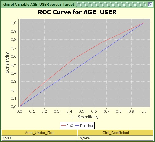
Image:Gini of grouped AGE versus Target
Notice the new variable now appears at the right end of the table under the menu bar. You can also see that that we came up with a pretty good uplift from 3.75% to 16.5% Gini, not bad. This uplift was a product of careful visualization of the 10-bin histogram we saw earlier. However, how do we know that we extracted the maximum information we could from those bins? Could we gain more if we scrutinize it better? The answer to the latter yes, but it can be quite a lengthy and time-consuming process to find those bins that can give you the maximum Gini. However kazAnova has tools that can do that for you given some constraints.
- Go to the Pre-process tab in the menu bar and press bin.
- In the only available column, select AGE or Type AGE in the second text field from the top.
- Change the name of the potential new variable in the first text field from the top to AGE_Optimised from AGE_derived.
- Press the fourth button from the top “MM’s Optimized Binning (Odds)”.
- In the only available column, select Target or Type Target in the first text field from the top.
- You can get different results by playing with some of those fields, but I will leave that to you to explore, for now just press “Apply” and close the pre-process tab.
- Save.
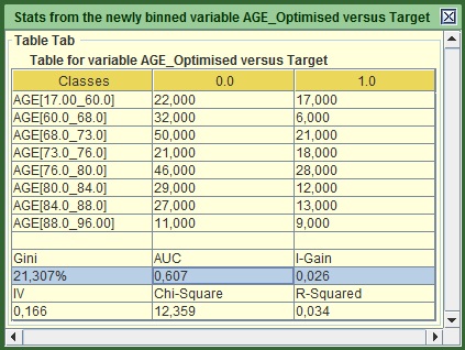
Image:Output of AGE after being optimized via ddds.
A new frame appears that shows the created bins, how many churners and non-churners exist in each bin and many of the statistics that we mentioned in the previous section. The new Gini is now 21.3% and constitutes a huge uplift in comparison to the 3.7% that it had when it was un-binned. Note that from the Bins, the right Value is always included, but the left value is not. E.g. AGE 68 would belong in AGE[60.0_68.0] not in AGE[68.0_73.0].
Time to bin HOURS and QUANTITY:
- Go to the Pre-process tab in the menu bar and press bin.
- In the only available column, select HOURS or Type HOURS in the second text field from the top.
- Change the name of the potential new variable in the first text field from the top to HOURS_Optimised from HOURS _derived. P.S. if you press the column, but the name appears differently in the text field, do not worry, just close the Pre-process tab and do it again.
- Press the fifth button from the top “MM’s Optimized Binning (Iv)”.
- On the only available column, select Target or Type Target in the first text field from the top.
- Do not change anything and press “Apply” and close the pre-process tab.
- Save.
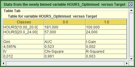
Image:Output of HOURS after being optimized via Information Value (IV).
Same for QUANTITY:
- Go to the Pre-process tab in the menu bar and press bin.
- In the only available column, select QUANTITY or Type QUANTITY in the second text field from the top.
- Change the name of the potential new variable in the first text field from the top to QUANTITY _Optimised from QUANTITY _derived.
- Press the sixth button from the top “MM’s Optimized Binning (Gini)”.
- On the only available column, select Target or Type Target in the first text field from the top.
- Do not change anything and press “Apply”.
- Save.
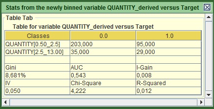
Image:Output of QUANTITY after being optimized via Gini.
These variables are ready for modeling. It is a good time to revisit some of the old String variables.
- Go to the Graphs tab in the menu bar and press Bar
 .
. - In the left of the two columns, select DISEASE or type DISEASE in the first text field from the top and in the right column select Target or type Target in the second text from the top.
- Press confirm.
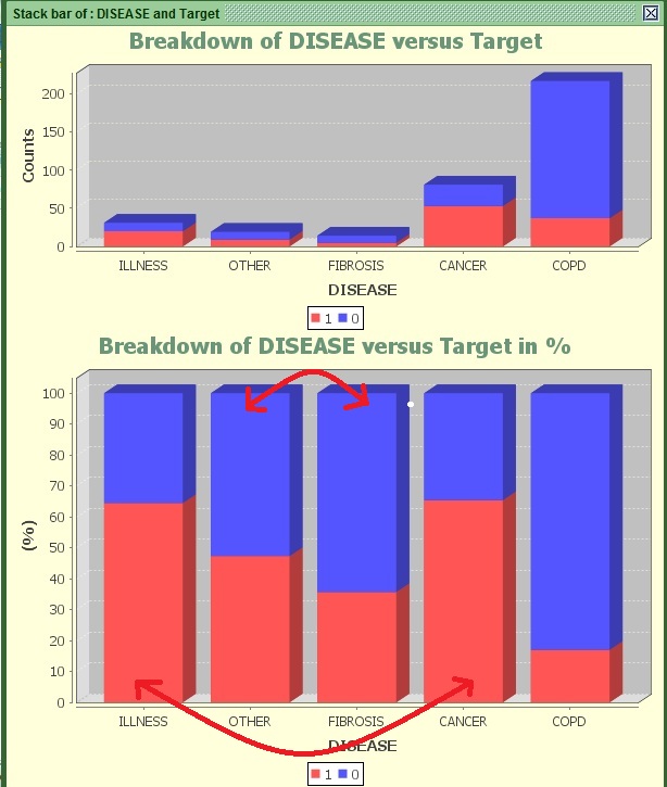
Image:Stack bar of DISEASE versus Target with suggestions.
You can see that ILLNESS and CANCER have similar propensity levels. Additionally OTHER and FIBROSIS have a small difference. Generally it is a good practice , especially in small sets like this one to merge some values together in order to increase their significance , promoting simplicity at the same time if it does not come at a cost of losing significant information .
In order to merge the values:
- Go to the Pre-process tab in the menu bar and press String-ing
 .
. - In the only available column, select DISEASE or Type DISEASE in the first text field from the top.
- Press the fifth button from the top “Bin String”.
In the new window that appears you can see the values of the DISEASE variable as a list on your left hand side:
- In the only available column, select CANCER and ILLNESS , or type CANCER, ILLNESS in the second text field from the top (the first one after the bar chart) .You may remove the “None,” part, but it does not really make any difference.
- In the Third text field from the top (the second one after the bar chart) . Remove the “None” part and put CANCER_ILLNESS.
- Press “ADD”.
- See that the graph changed and you can now see only 4 values, including the one you just created.
- Select FIBROSIS and OTHER, or type FIBROSIS, OTHER in the second text field from the top (the first one after the bar chart).
- In the Third text field from the top (the second one after the bar chart) put FIBROSIS_ OTHER.
- Press “ADD”.
- Finally, in the new frame that appears put the name DISEASE_SHORT in the first text field from the top (Before the bar chart)
- Press “Apply”.
- Save the drowning guy.
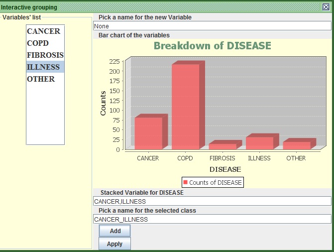
Image:Merging CANCER with ILLNESS in the Bin String section
We shall do the same for FIBROSIS and OTHER:
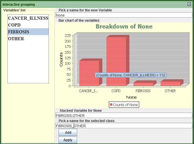
Image:Merging FIBROSIS with OTHER in the Bin String section
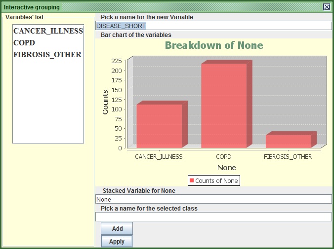
Image:Finalize Merging by pressing Apply.
You can see that a new frame appears that shows the counts and the proportions of the classes. If you now check the Gini again, you will see that it is 48.64% in comparison to 48.82% that was before. We have essentially lost almost nothing, but we made the variable much more significant and the future results more solid by boosting the frequencies of the classes.
Again, that was fairly easy to catch with the eye, what if we had many variables with many classes. It would be very time consuming…Do not worry, because again kazAnova can do this for you!
- Go to the Pre-process tab in the menu bar and press String-ing.
- On the only available column, select DISEASE or Type DISEASE in the first text field from the top.
- Press the last button from the top “Optimisation Binning”.
- On the only available column, select Target or Type Target in the second text field from the top (the first one after the graph).
- Leave the name in the first text field as it is DISEASE_Optimised.
- Put desired number of bins value to 3 (third text field).
- Press the second button “Optimize(Gini)”. Parenthesis, you will notice that at some points I put Optimize with “z” and other times with “s”. I still don’t know why I do that. Actually I figured that just right now, end of Parenthesis.
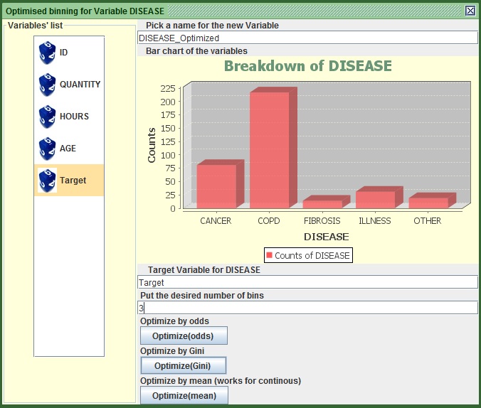
Image:Optimize DESEASE via Gini.
The new frame that appears shows the counts and the calculated statistics. You will notice that it has binned the variable in exactly the same way we did before.
At this point you might want to create some new variables, but I will leave that for now in order to make things simple. I will talk again about this at tutorial 6.
One last thing before we proceed is to split the set. Generally in modeling we have 2 basic sets, the training and the validation set. We use the training set to build the logic (to create the scores) and the validation to test it. In other words the validation set is never used in the process when we run the algorithm. In kazAnova this splitting, is just a variable that takes the values of 1 or 0. KazAnova puts the row that has the value of 1 in the training set and anything that has 0 to the validation set. To create one such variable:
- Go to the Pre-process tab in the menu bar and press “Sampling”
 .
. - In the new frame, change the name in the second text field from the top from “partition001” to partition_simple.
- Note the split value is 0.5. This means that 50% will be in the training and 50% in the validation.
- Press “Compute”.
- Save yesterday.
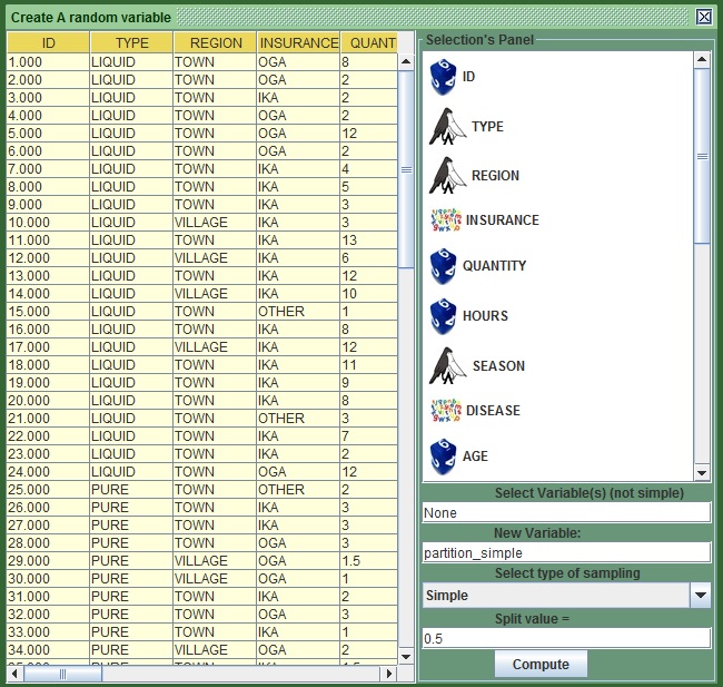
Image:Create a partition variable
An interesting thing to know is that the splitting method allows you to do a variable-based splitting. For example if you choose “Variable-based” in the scroll down menu and choose the Target variable, the training and validation set will try to have the same number proportionally of churners and non-churners. That is particularly good when the count of your basic category (e.g. churners) is rather small.
We made some good progress; we are ready to create our first scorecard however we are not going to use all the nice variables that we created to make it easier for someone to follow up from that point. You may now proceed to tutorial 4.